Hide code cell content

import mmf_setup; mmf_setup.nbinit()
import os
from pathlib import Path
FIG_DIR = Path(mmf_setup.ROOT) / '../Docs/_build/figures/'
os.makedirs(FIG_DIR, exist_ok=True)
import logging; logging.getLogger("matplotlib").setLevel(logging.CRITICAL)
%matplotlib inline
import numpy as np, matplotlib.pyplot as plt
try: from myst_nb import glue
except: glue = None

This cell adds /home/docs/checkouts/readthedocs.org/user_builds/iscimath-581-estimation/checkouts/latest/src to your path, and contains some definitions for equations and some CSS for styling the notebook. If things look a bit strange, please try the following:

  • Choose "Trust Notebook" from the "File" menu.
  • Re-execute this cell.
  • Reload the notebook.

Dirac Delta Function#

Physicists often use Dirac’s delta function \(\delta(x)\) to express various quantities. Here are various formulations with increasing degree of rigor.

As a Function#

Hide code cell source

x = [-1, 0, 0, 0, 1]
y = [0, 0, 1, 0, 0]
fig, ax = plt.subplots(figsize=(3, 2))
ax.plot(x, y, 'C0-', zorder=0)
ax.scatter([0], [0], edgecolors='C0', facecolors='w', zorder=1)
ax.set(xlabel="$x$", xticks=[-1, 0, 1], 
       ylabel=r"$\delta(x)$", yticks=[0,1], yticklabels=["$0$", r"$\infty$"]);
../_images/c362560e0b6f6ade0c5f978ab186079cf7b98674fac064942096cf430d0da2fd.png

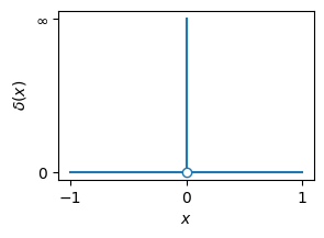
We often treat \(\delta(x)\) as a function

\[\begin{gather*} \delta(x) = \begin{cases} \infty & x = 0,\\ 0 & x \neq 0, \end{cases} \end{gather*}\]

where the value \(\infty\) at \(x=0\) is such that the area is 1.

\[\begin{gather*} \int_{-\epsilon}^{\epsilon} \delta(x)\d{x} = 1, \qquad \int_{-\infty}^{\infty} f(x)\delta(x-x_0)\d{x} = f(x_0). \end{gather*}\]

Well, convenient, this representation is incomplete a \(\delta(x)\) is not a function in any real sense.

Counterexample

Consider the meaning of \([\delta(x)]^2\).

Hide code cell content

from IPython.display import HTML, Javascript, display
from matplotlib import animation
plt.rcParams["animation.html"] = "jshtml"

epsinvs = np.arange(1, 16)
fig, ax = plt.subplots(figsize=(4/2, 8/2))

def animate(epsinv):
    global ax

    eps = 1/epsinv
    ax.cla()
    ax.set(xlim=(-2, 2), xlabel="$x$", xticks=[-2, -1, 0, 1, 2], 
           ylim=(-1, 8), ylabel=r"$\delta_{\epsilon}(x)$",
           title=fr"$\epsilon = 1/{epsinv}$")
    x = np.linspace(-2, 2, 100)
    y = np.exp(-(x/eps)**2)/np.sqrt(eps**2*np.pi)
    ax.plot(x, y, 'C0-')
    y = np.sin(x/eps)/np.pi/x
    ax.plot(x, y, 'C2-')
    y = np.sin((1/eps+0.5)*x)/np.sin(x/2)/2/np.pi
    ax.plot(x, y, 'C3-')
    y = 1/(1+(x/eps)**2)/eps/np.pi
    ax.plot(x, y, 'C4-')
    h = 2*eps
    ax.plot([-2, -h], [0, 0], 'C1-')
    ax.plot([-h, h], [1/h, 1/h], 'C1-')
    ax.plot([h, 2], [0, 0], 'C1-')
    ax.plot([-h, -h], [0, 1/h], 'C1:')
    ax.plot([h, h], [0, 1/h], 'C1:')
    return ax,

anim = animation.FuncAnimation(fig, animate, repeat=True, frames=epsinvs, interval=500)

# To save the animation using Pillow as a gif
anim.save(FIG_DIR / 'delta_function1.gif', writer=animation.PillowWriter(fps=5))
../_images/d792e1584fe99870b198213e93c3ddad360eff332e1a66c880da98cf56d62260.png
../_images/delta_function1.gif

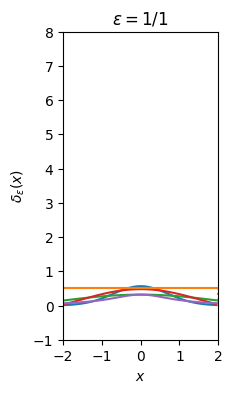
Fig. 1 Representing \(\delta(x) = \lim_{\epsilon\rightarrow 0}\delta_{\epsilon}(x)\) as a limit of functions. The step function here has \(\epsilon \rightarrow 2\epsilon\) for better visual comparison, otherwise the formula are as given in the text.#

As a Limit or Distribution#

One way to make this idea rigorous is to think of \(\delta(x)\) as a limit of appropriate functions where the limit is taken outside of the calculation. For example

\[\begin{gather*} \delta(x) \equiv \lim_{\epsilon\rightarrow 0} \delta_{\epsilon}(x), \qquad \int\delta(x)f(x)\d{x} = \lim_{\epsilon\rightarrow 0}\int\delta_{\epsilon}(x)f(x)\d{x}. \end{gather*}\]

Some suitable examples of \(\delta_{\epsilon}(x)\) sequences are:

\[\begin{align*} \delta_{\epsilon}(x) &= \frac{1}{\abs{\epsilon}}\begin{cases} 1 & \abs{x} < \epsilon,\\ 0 & \text{otherwise}, \end{cases},\\ \delta_{\epsilon}(x) &= \frac{1}{\abs{\epsilon}\sqrt{\pi}}e^{-(x/\epsilon)^2},\\ \delta_{\epsilon}(x) &= \frac{1}{\abs{\epsilon}\pi}\frac{1}{1+(x/\epsilon)^2},\\ \delta_{\epsilon}(x) &= \frac{\sin x/\epsilon}{\pi x} = \frac{1}{2\pi}\int_{-\epsilon^{-1}}^{\epsilon^{-1}}e^{\I k x}\d{k}. \end{align*}\]

The last form is sometimes expressed as the Dirichlet kernel

\[\begin{gather*} \delta_{1/n}(x) = \frac{1}{2\pi}\frac{\sin\bigl[(n+\tfrac{1}{2})x\bigr]} {\sin(\tfrac{1}{2}x)}. \end{gather*}\]

If the limit exists, then it will be independent of the form of \(\delta_{\epsilon}(x)\).

Interpreted this way, \(\delta(x)\) is sometimes called a distribution.

Riemann-Stieltjes Integral#

Another rigorous definition is in terms of a Riemann-Stieltjes Integral:

\[\begin{gather*} \int f(x)\d{g(x)} = \int f(x)g'(x)\d{x}, \end{gather*}\]

where \(g(x)\) is differentiable. The Riemann-Stieltjes Integral remains valid even \(g(x)\) is discontinuous, and the delta-function can be expressed in terms of the Heaviside step function \(H(x)\):

\[\begin{gather*} f(x_0) = \int f(x) \d{H(x-x_0)}, \qquad H(x) = \begin{cases} 1 & x >0,\\ \tfrac{1}{2} & x = 0,\\ 0 & x < 0. \end{cases} \end{gather*}\]

Note that, informally, \(\delta(x) = H'(x)\), reproducing the informal notation above.

Example

In class, we discussed the informal result

\[\begin{gather*} \delta\bigl(g(x)-g_0)\bigr) = \sum_{x_i \in g^{-1}(g_0)}\frac{\delta(x-x_i)}{\abs{g'(x_i)}},\\ \int f(x)\delta\bigl(g(x)-g_0)\bigr)\d{x} = \sum_{x_i \in g^{-1}(g_0)} \frac{f(x_i)}{\abs{g'(x_i)}},\\ g^{-1}(g_0) = \{x_i \; |\; g(x_i) = g_0\}. \end{gather*}\]

We can express this as

\[\begin{gather*} \int f(x)\d{M(x)}, \qquad M(x) = \sum_{x_i \in g^{-1}(g_0)}\frac{H(x-x_i)}{\abs{g'(x_i)}}. \end{gather*}\]

Kevin has some additional notes (PDF).