Drag

Drag#

In class, we explored the following model for drag force:

\[\begin{gather*} F_{d} \approx 2\rho_{\text{air}} A v^2 \sin^{\alpha}\theta \end{gather*}\]

where \(\rho_{\text{air}}\) is the mass-density of air, \(A\) is the cross-sectional area, \(v\) is the falling speed, and \(\theta\) is the cone half-angle. We expect \(\alpha = 1\), but the question is: using simple resources available in class, can we reasonably test the hypothesis that \(\alpha = 1\)?

Here we present some results for analyzing this model.

Quantities

Dynamic viscosity of air:

\[\begin{gather*} \eta_{\text{air}} \approx 18.5\; \mathrm{\mu Pa\cdot s} \left(\frac{T}{300\mathrm{K}}\right)^{0.7}. \end{gather*}\]

Terminal Velocity#

We first simplify the model to express the drag force as

\[\begin{gather*} F_{d} = \beta v^2, \qquad \beta \approx 2\rho_{\text{air}} A \sin^{\alpha}\theta. \end{gather*}\]

Newton’s law gives the terminal velocity when \(\dot{v} = 0\):

\[\begin{gather*} m\dot{v} = mg - F_d = mg - \beta v^2, \qquad v_T = \sqrt{\frac{mg}{\beta}} \approx \sqrt{\frac{mg}{2\rho_{\text{air}} A \sin^{\alpha}\theta}}. \end{gather*}\]

Do It!

Think about this form. We can test several things. First, our model posits that the drag force depends quadratically on the velocity. Can you test this from your data? Next we have the dependence on the cone angle: will your results be sensitive enough to test this? Do a dimensional analysis: is there a dimensionless parameter?

This analysis has ignored the viscosity of the air: include \(\eta_{\text{air}}\) in your analysis.

It might be difficult in class to ensure that the cones are measured only during the time when they reach \(v_T\), so we may want to determine the average velocity after falling through a time \(t\) or height \(h\).

To do this, we choose units so that \(v_T = m = g = 1\):

\[\begin{gather*} 1 = \underbrace{m}_{\text{mass}} = \underbrace{\frac{v_T}{g}}_{\text{time}} = \underbrace{\frac{v_T^2}{g}}_{\text{distance}} = \underbrace{v_T}_{\text{speed}}. \end{gather*}\]

With these units, we have:

\[\begin{gather*} \dot{v} = 1 - v^2\\ \int_{0}^{v}\frac{1}{1-v^2}\d{v} = \int_0^{t}\d{t}, \qquad \frac{1}{2}\ln\frac{1+v}{1-v} = t, \qquad 1+v = (1-v)e^{2t},\\ v = \frac{e^{2t} - 1}{e^{2t} + 1} = \frac{e^{t} - e^{-t}}{e^{t} + e^{-t}} = \tanh t,\\ h = \int_0^{t}\d{t}\;\tanh t = t - \ln\bigl(1+\tanh(t)\bigr). \end{gather*}\]

from scipy.integrate import solve_ivp
def dv_dt(t, v):
    return 1-v**2
res = solve_ivp(dv_dt, t_span=(0, 3), y0=[0], max_step=0.1)
t, v = res.t, res.y[0]
assert np.allclose(v, np.tanh(t))
h = t - np.log(1+np.tanh(t))

fig, axs = plt.subplots(1, 2, figsize=(8, 3))
ax = axs[0]
ax.plot(t, v, label="solve_ivp")
ax.plot(t, np.tanh(t), label="exact")
ax.plot(t, h/t, label="$h/t$")
ax.legend()
ax.set(xlabel="$t$ [$v_T/g$]", ylabel="$v$ [$v_T$]");
ax = axs[1]
ax.plot(t, h)
ax.set(xlabel="$t$ [$v_T/g$]", ylabel="$h$ [$v_T^2/g$]")
plt.tight_layout();

/tmp/ipykernel_3861/131946542.py:13: RuntimeWarning: invalid value encountered in divide
  ax.plot(t, h/t, label="$h/t$")

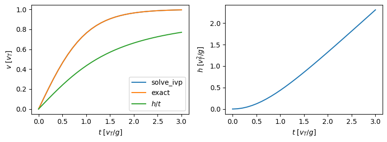
../_images/a7eda0e0e59f14c7ca9949079a1a622d019ed6b81fa5677c0722b11f3b08cb82.png

We see from the plot that the falling object will reach terminal velocity within about 2-3 time units \(v_T/g\).

Sample Data#

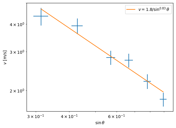
Here we analyze a set of data from one of the groups. The data here is a list of terminal velocities \(v\) correlated with \(\sin\theta\):

from uncertainties import ufloat, unumpy as unp

m = ufloat(1.6, 0.1)*1e-3
base_diameter = [9.4e-2, 8.2e-2, 7e-2, 6e-2, 4.5e-2, 3.3e-2]
dr = 0.001  # Error in table?
r = np.array([ufloat(d/2, dr) for d in base_diameter])
side_length = ufloat(5.25e-2, 0.1e-2)
v_terminal = np.array([ufloat(*v) for v in [
    (1.82, 0.13),
    (2.20, 0.17),
    (2.74, 0.20), 
    (2.82, 0.21),
    (3.93, 0.32),
    (4.35, 0.40)]])
sin_thetas = r/side_length

_n, _s = unp.nominal_values, unp.std_devs
fig, ax = plt.subplots()
ax.errorbar(_n(sin_thetas), _n(v_terminal), ls='none', 
            xerr=_s(sin_thetas), yerr=_s(v_terminal))
ax.set(xlabel=rf"$\sin\theta$", ylabel="$v$ [m/s]",
       xscale="log", yscale="log");
a, b = np.polyfit(np.log(_n(sin_thetas)), np.log(_n(v_terminal)), deg=1)

x_ = _n(sin_thetas)
th = np.linspace(np.asin(x_.min()), np.asin(x_.max()))
x = np.sin(th)
y = np.exp(b)*x**a
ax.plot(x, y, label=fr"$v = {np.exp(b):.2g}/\sin^{{{-a:.2g}}}\theta$")
ax.legend()

<matplotlib.legend.Legend at 0x734e64a9e910>

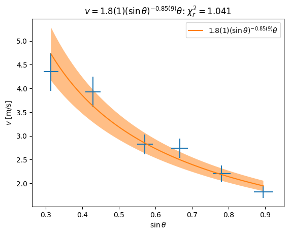
../_images/1896dcd8cadf14cc1534f533ce21ea37dd8010b73fd26cc8e9300311a9115012.png

Quantitative Analysis#

In this case, to search for a power-law dependence, we can just do a linear regression of the appropriate variables as we plotted above, but we will present this as a general fit to demonstrate how you might do this for more complicated models.

We can start with scipy.optimize.curve_fit(), which fits

\[\begin{gather*} y = f(x, p_1, p_2, \dots) + \epsilon, \qquad \epsilon \sim \mathcal{N}_{\sigma} \end{gather*}\]

where the errors \(\epsilon\) are assumed to be normally distributed with standard deviation \(\sigma\). This does not allow us to model the errors in \(x\), but we can get an estimate of the uncertainties.

We will use the model

\[\begin{gather*} y = v = ax^{\alpha}, \qquad x = \sin \theta. \end{gather*}\]

from scipy.optimize import curve_fit

def f(sin_theta, a, alpha):
    return a * sin_theta**alpha

xdata = _n(sin_thetas)
ydata = _n(v_terminal)
sigma = _s(v_terminal)
p0 = [1.0, 1.0]  # Initial guess
res = curve_fit(
    f, xdata=xdata, ydata=ydata, sigma=sigma,
    absolute_sigma=True,  # Assume the stated errors are correct
    )
popt, pcov = res
perr = np.sqrt(np.diag(pcov))
a = ufloat(popt[0], perr[0])
alpha = ufloat(popt[1], perr[1])

# Reduced chi^2
chi2r = np.sum((abs(ydata - f(xdata, *popt))/sigma)**2)/(len(xdata) - len(popt))

fig, ax = plt.subplots()
ax.errorbar(xdata, ydata, ls='none', 
            xerr=_s(sin_thetas), yerr=_s(v_terminal))
x = sin_th = np.linspace(xdata.min(), xdata.max())
y = f(x, a=a, alpha=alpha)
l, = ax.plot(x, _n(y), label=fr"${a:.2S}(\sin\theta)^{{{alpha:.2S}}}\theta$")
ax.fill_between(x, _n(y)-_s(y), _n(y)+_s(y), fc=l.get_c(), alpha=0.5)
ax.legend()
ax.set(xlabel=rf"$\sin\theta$", ylabel="$v$ [m/s]", 
       title=fr"$v = {a:.2S}(\sin\theta)^{{{alpha:.2S}}}\theta$: $\chi^2_r = {chi2r:.4g}$");

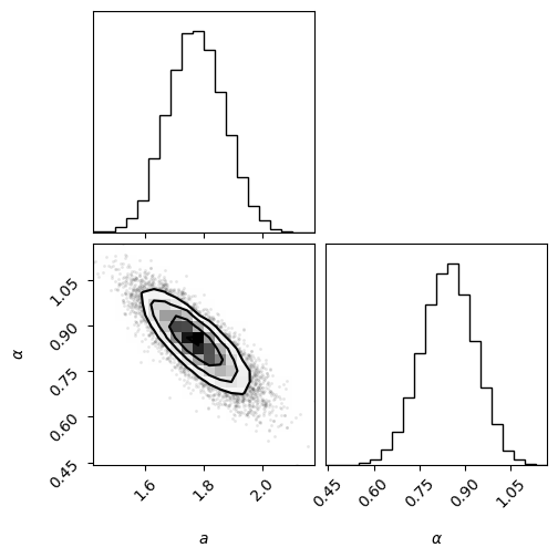
../_images/7c9fe84e5b4ac7cb0278eb13393ace803b0a1a6bee75f49d7fba894d16460d88.png

Bayesian Analsyis#

Now let’s do this with Bayesian analysis. For now we will ignore the errors in the abscissa. Our model is thus

\[\begin{gather*} v_t = a\sin^{-\alpha} \theta + \epsilon \end{gather*}\]

where the errors \(\epsilon\) are assumed to have a known distribution \(p(\epsilon)\) which we take to be Gaussian

\[\begin{gather*} p_{\epsilon}(\epsilon) \propto e^{-\epsilon^2/2/\sigma^2}. \end{gather*}\]

We also need a prior \(p_0(a, \alpha)\). If we do not know anything, we might choose an uninformed prior \(p_0(a, \alpha) \propto 1\). Note: this is not normalizable… we will deal with this later.

Now we apply Bayes theorem to determine the posterior distribution:

\[\begin{gather*} p(a, \alpha|D) \propto p(D|a, \alpha)p_0(a, \alpha) \end{gather*}\]

where the likelihood \(p(D|a, \alpha)\) is the probability of obtaining the data \(D\) given a fixed set of parameters \(a\) and \(\alpha\). In our case, this is exactly what we mean by the estimated error \(\epsilon\):

\[\begin{gather*} \epsilon = v_t -a\sin^{-\alpha} \theta,\\ p(D|a, \alpha) = p_{\epsilon}(\epsilon) = p_{\epsilon}\Bigl(v_t -a\sin^{-\alpha} \theta\Bigr). \end{gather*}\]

For multiple data points, we would take the product over all data points. For example, consider two data points:

\[\begin{gather*} p(a, \alpha|D_1, D_2) \propto p(D_2|a, \alpha)\underbrace{p(D_1|a, \alpha)p_0(a, \alpha)}_{p(a, \alpha | D_1)}. \end{gather*}\]

Note that this has a simple interpretation: the bracketed quantity – what we learn after taking one measurement – becomes the prior for adding the second measurement. As long as everything is uncorrelated, the order in which we add the data does not matter.

With gaussians, and flat priors etc., you can do everything analytically (Do It!) but here we will do it numerically with the emcee package so we can generalize. This package works with the log of everything, so we have

\[\begin{gather*} \log p(a, \alpha| D) \propto \log p(D|a, \alpha) + \log p(a, \alpha). \end{gather*}\]

To use the code, you must write the right-hand-side function. In our case:

\[\begin{gather*} \log p(a, \alpha| D) \propto \sum_{n} \log p_{\epsilon}\Bigl(v_n -a\sin^{-\alpha} \theta_n\Bigr) + \log p_0(a, \alpha). \end{gather*}\]

For gaussian errors, and constant prior, this is exactly the negative \(\chi^2\) usually used for curve fitting:

\[\begin{gather*} \log p(a, \alpha| D) \propto - \underbrace{\sum_{n} \frac{\Bigl(v_n -a\sin^{-\alpha}\theta_n\Bigr)^2}{2\sigma^2}}_{\chi^2} + \log p_0(a, \alpha). \end{gather*}\]

import emcee

def log_prior(a, alpha):
    return 0.0  # Uninformed
    
def log_probability(params, sin_theta, v, v_err):
    a, alpha = params
    eps = (v - a/sin_theta**alpha)
    sigma = v_err
    return -0.5 * np.sum((eps/sigma)**2)

rng = np.random.default_rng(seed=2)
nwalkers = 32
ndim = 2
guess = np.array([1.8, 0.83]) + rng.normal(size=(nwalkers, ndim))

sampler = emcee.EnsembleSampler(
    nwalkers, ndim, log_probability, 
    args=(_n(sin_thetas), _n(v_terminal), _s(v_terminal)))

sampler.run_mcmc(guess, 5000, progress=False);

Now that we have run our sampler, we can estimate the autocorrelation times:

tau = sampler.get_autocorr_time()
print(tau)

[31.925001   29.53996664]

These suggest that we only need about 30 steps to remove any spurious correlations from the initial data. We then include every 15th sample (about half the autocorrelation time). Finally, we flatten the samples so we can pass it to the plotting routine.

flat_samples = sampler.get_chain(discard=100, thin=15, flat=True)
print(flat_samples.shape)

(10432, 2)

import corner

fig = corner.corner(flat_samples, labels=("$a$", r"$\alpha$"))

../_images/f89e1a657f70a6fa0afa08b75f886583a96e360be4eedbd8907462df191460fe.png

Errors in the Abscissa#

So far we have neglected the errors in \(\sin\theta\). Here we fix this. The idea is to consider the half-angle \(\theta_i\) as a another parameter: we are trying to make cones with this half-angle, but we then measure the cones and obtain values \(x_i\) that deviate from \(\sin \theta_i\) by a random amount \(\delta_i\). Thus, our complete error model is:

\[\begin{gather*} v_{i} = \frac{a}{\sin^\alpha \theta_i} + \epsilon_i, \\ x_{i} = \sin \theta_i + \delta_i. \end{gather*}\]

If these errors are independent, then the likelihood is the product

\[\begin{gather*} p_{\epsilon_{i}}\Bigl(v_{i} - \frac{a}{\sin^\alpha \theta_i}\Bigr) p_{\delta_{i}}\Bigl(x_{i} - \sin\theta_i\Bigr). \end{gather*}\]

We must now include the abscissa \(\vect{\theta}\) as additional parameters. Following through Bayes’s theorem, we end up with a posterior \(p(a, \alpha, \vect{\theta}|D)\). Explicitly, for a single data point

\[\begin{gather*} p(a, \alpha) \propto p_{\epsilon}\Bigl(v - \frac{a}{\sin^\alpha \theta}\Bigr) p_{\delta}\Bigl(x - \sin\theta\Bigr)p_0(a, \alpha, \theta). \end{gather*}\]

Now, we don’t really care about the values of \(\vect{\theta}\) – they are nuisance parameters. To obtain the posterior distribution of \(a\) and \(\alpha\), we should marginalize over these by integrating:

\[\begin{gather*} p(a, \alpha|D) = \int p(a, \alpha, \vect{\theta}|D)\d\vect{\theta}. \end{gather*}\]

While this seems tricky analytically, it is trivial with samples – simply ignore the nuisance variables!